next up previous
Next: Bibliography

A Posteriori Error Analysis for Nonstandard FEM

Carsten Carstensen

General strategies are discussed to derive a posteriori error estimates for conforming, mixed, and nonconforming finite element methods in energy norms which also cover discontinuous Galerkin schemes or Mortar finite elements for second order elliptic problems. The unifying approach provides reliable error estimates which can be shown to be efficient as well. One may say that all nonstandard schemes allow for error control, there is no finite element method known to the author where there is no error control. 
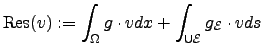
Surprisingly, there remains one type of residuals $ {\mathrm{Res}}$ for different problems, such as, the Laplace problem, the Stokes problem, and Navier-Lamé problem. The main observation is that

$\displaystyle {\mathrm{Res}}(v):=\int_{\Omega}g\cdot v dx +\int_{\cup\ensuremath{\mathcal{E}} }g_{\ensuremath{\mathcal{E}} }\cdot v ds$    for $\displaystyle v \in V
$

is the same for all those schemes. Some nonconforming elements are depicted in the following tables.
picture name

\begin{picture}(15,15)
\put(0,0){\line(1,0){10}} \put(0,0){\line(1,2){5}}
\put...
...0){\circle*{2}}
\put(2.5,5){\circle*{2}} \put(7.5,5){\circle*{2}}
\end{picture}
Crouzeix-Raviart

\begin{picture}(15,15)
\put(0,0){\line(1,0){10}} \put(0,0){\line(0,1){10}}
\pu...
...0){\circle*{2}}
\put(5,3.3){\circle*{2}} \put(5,6.6){\circle*{2}}
\end{picture}
Wilson

\begin{picture}(15,15)
\put(0,0){\line(1,0){10}} \put(0,0){\line(0,1){10}}
\pu...
...(5,10){\circle*{2}} \put(0,5){\circle*{2}}
\put(5,5){\circle*{2}}
\end{picture}
Han

\begin{picture}(15,15)
\put(0,0){\line(1,0){10}} \put(0,0){\line(0,1){10}}
\pu...
...1){7}}
\put(10,10){\vector(-1,0){7}} \put(0,10){\vector(0,-1){7}}
\end{picture}
NR (M)

\begin{picture}(15,15)
\put(0,0){\line(1,0){10}} \put(0,0){\line(0,1){10}}
\pu...
...10,5){\circle*{2}}
\put(5,10){\circle*{2}} \put(0,5){\circle*{2}}
\end{picture}
NR (A)

\begin{picture}(15,15)
\put(0,0){\line(1,0){10}} \put(0,0){\line(0,1){10}}
\pu...
...,0){\circle*{2}}
\put(10,10){\circle*{2}} \put(0,10){\circle*{2}}
\end{picture}
CNR

\begin{picture}(15,15)
\put(0,0){\line(1,0){10}} \put(0,0){\line(0,1){10}}
\pu...
...10,5){\circle*{2}}
\put(5,10){\circle*{2}} \put(0,5){\circle*{2}}
\end{picture}
DSSY

picture name

\begin{picture}(15,15)
\put(0,0){\line(1,0){10}} \put(0,0){\line(1,2){5}}
\put...
...{\circle*{2}}
\put(14.5,5){\circle*{2}} \put(19.5,5){\circle*{2}}
\end{picture}
Crouzeix-Raviart

\begin{picture}(15,15)
\put(0,0){\line(1,0){10}} \put(0,0){\line(1,2){5}}
\put...
...{\circle*{2}}
\put(14.5,5){\circle*{2}} \put(19.5,5){\circle*{2}}
\end{picture}
Kouhia-Stenberg

\begin{picture}(15,15)
\put(0,0){\line(1,0){10}} \put(0,0){\line(0,1){10}}
\pu...
...,10){\circle*{2}} \put(13,5){\circle*{2}}
\put(18,5){\circle*{2}}
\end{picture}
Han

\begin{picture}(15,15)
\put(0,0){\line(1,0){10}} \put(0,0){\line(0,1){10}}
\pu...
...){7}}
\put(23,10){\vector(-1,0){7}} \put(13,10){\vector(0,-1){7}}
\end{picture}
NR (M)

\begin{picture}(15,15)
\put(0,0){\line(1,0){10}} \put(0,0){\line(0,1){10}}
\pu...
...,5){\circle*{2}}
\put(18,10){\circle*{2}} \put(13,5){\circle*{2}}
\end{picture}
NR (A)

\begin{picture}(15,15)
\put(0,0){\line(1,0){10}} \put(0,0){\line(0,1){10}}
\pu...
...0){\circle*{2}}
\put(23,10){\circle*{2}} \put(13,10){\circle*{2}}
\end{picture}
HMS

\begin{picture}(15,15)
\put(0,0){\line(1,0){10}} \put(0,0){\line(0,1){10}}
\pu...
...,5){\circle*{2}}
\put(18,10){\circle*{2}} \put(13,5){\circle*{2}}
\end{picture}
CJY

picture name

\begin{picture}(15,15)
\put(0,0){\line(1,0){10}} \put(0,0){\line(1,2){5}}
\put...
...{\circle*{2}}
\put(14.5,5){\circle*{2}} \put(19.5,5){\circle*{2}}
\end{picture}
Brenner-Sung

\begin{picture}(15,15)
\put(0,0){\line(1,0){10}} \put(0,0){\line(1,2){5}}
\put...
...{\circle*{2}}
\put(14.5,5){\circle*{2}} \put(19.5,5){\circle*{2}}
\end{picture}
Kouhia-Stenberg

\begin{picture}(15,15)
\put(0,0){\line(1,0){10}} \put(0,0){\line(0,1){10}}
\pu...
...{\circle*{2}}
\put(18,3.3){\circle*{2}} \put(18,6.6){\circle*{2}}
\end{picture}
Zhang

\begin{picture}(15,15)
\put(13,0){\line(1,0){10}} \put(13,0){\line(0,1){10}}
\...
...,0){\circle*{2}}
\put(10,10){\circle*{2}} \put(0,10){\circle*{2}}
\end{picture}
Ming

\begin{picture}(15,15)
\put(0,0){\line(1,0){10}} \put(0,0){\line(0,1){10}}
\pu...
...,5){\circle*{2}}
\put(18,10){\circle*{2}} \put(13,5){\circle*{2}}
\end{picture}
LLS

\begin{picture}(15,15)
\put(0,0){\line(1,0){10}} \put(0,0){\line(0,1){10}}
\pu...
...0){\circle*{2}}
\put(23,10){\circle*{2}} \put(13,10){\circle*{2}}
\end{picture}
HMS

     
NCFEM for Laplace NCFEM for Stokes NCFEM for Navier-Lamé

Several discontinuous Galerkin methods are analysed in the same unifying framework and the subsequent tables display a few examples. The unifying notation due to Cockburn and Shu is not recalled but employed to specify the methods which are not properly labelled in this abstract.


Table: dG schemes and their specifications for LAPLACE
Method [Ref.] $ \hat u_T$ $ \hat p_T$ $ c_1$ $ c_2 $
         
Bassi-Rebay (1997) $ \{u_h\}$ $ \{p_h\}$ -1 0
Brezzi et MMPR (1999) $ \{u_h\}$ $ \{p_h\}-\alpha_r(\underline{[u_h]})$ -1 0
LDG of CS (1998) $ \{u_h\}-\beta\cdot
\underline{[u_h]} $ $ \{p_h\}+\beta[\sigma_h]-\alpha_j(\underline{[u_h]}) $ -1 0
IP of DD (1976) $ \{u_h\}$ $ \{D u_h\}-\alpha_j(\underline{[u_h]})$ -1 0
Bassi et RMPS (1997) $ \{u_h\}$ $ \{D u_h\}-\alpha_r(\underline{[u_h]})$ -1 0
Baumann-Oden (1999) $ \{u_h\}+\nu_T\cdot
\underline{[u_h]}$ $ \{D u_h\}$ 1 0
NIPG RWG (1999) $ \{u_h\}+\nu_T\cdot
\underline{[u_h]}$ $ \{D u_h\}-\alpha_j(\underline{[u_h]})$ 1 0
Babuska-Zlamal (1973) $ (u_h\vert _T)\vert _{\partial T}$ $ -\alpha_j(\underline{[u_h]})$ 0 0
Brezzi et MM (2000) $ (u_h\vert _T)\vert _{\partial T}$ $ -\alpha_r(\underline{[u_h]})$ 0 0


Table: dG schemes and their specifications for STOKES
Method [Ref.] $ \hat u_{T,\sigma}$ $ \hat u_{T,p}$ $ \hat\sigma_T$ $ c_1$ $ c_2 $
Bassi-Rebay (1997) $ \{u_h\}$ $ \{u_h\}$ $ \{\sigma_h\} $ -1 0
IP of SST (2003) $ \{u_h\}$ $ \{u_h\}$ $ \{D u_h\}-\alpha_j(\underline{[u_h]})$ -1 0
Bassi et RMMPR (1997) $ \{u_h\}$ $ \{u_h\}$ $ \{D u_h\}-\alpha_r(\underline{[u_h]})$ -1 0
NIPG of Toselli (2002) $ \{u_h\}+\underline{[u_h]}\cdot\nu_T$ $ \{u_h\}$ $ \{D u_h\}-\alpha_j(\underline{[u_h]})$ 1 0
LDG of GKSS (2002) $ \{u_h\}+\underline{[u_h]}\cdot\beta$ $ \{u_h\}+D_{11}[p_h]\newline +D_{12}[u_h]$ $ \{\sigma_h\}-[\sigma_h]\otimes\beta \newline -[p_h]
\otimes\beta \newline - D_{12}\cdot[p_h]-\alpha_j(\underline{[u_h]})$ -1 1


Table: dG schemes and their specifications for NAVIER LAME
Method $ \hat u_{T,\varepsilon}$ $ \hat u_{T,p}$ $ \hat\sigma_T$ $ \hat p_T$ $ c_1$ $ c_2 $
IP of HL (2002) $ \{u_h\}$ $ \{u_h\}$ $ \{\varepsilon(u_h)\}\newline -\alpha_j(\underline{[u_h]})$ $ -\lambda \{D\cdot u_h\}\newline +\lambda\alpha_j([u_h])$ 0 0
LDG of CKSS (2006) $ \{u_h\}+\underline{[u_h]}\cdot\beta$ $ \{u_h\}+D_{12}[u_h]\newline +D_{11}\underline{[p_h]}$ $ \{\varepsilon_h\}-[\varepsilon_h]\otimes\beta \newline -\alpha_j(\underline{[u_h]})$ $ \{p_h\}-D_{12}\cdot\underline{[p_h]}$ -1 1


The conclusion of this presentation is sparsity in the mathematical research of a posteriori error control. The reduction is to two parts. (a) Analyze your new PDE in such a way that the error is equivalent to $ \Vert{\mathrm{Res}}\Vert _{\ast}$ and analyze $ V_h\subset \ker {\mathrm{Res}}$. (b) Design new a posteriori error estimates for $ \Vert{\mathrm{Res}}\Vert _{\ast}$.

The presentation is partly based on joint work [1-4] with Jun Hu, Antinio Orlando, Max Jensen, and Thirupathi Gudi.


next up previous
Next: Bibliography
Tsorng-Whay Pan 2008-03-06