The mathematical model presented here is a nonlinear system of differential
equations describing the growth rate of the cell population with concentration
![]() , and
the growth rate of the extracellular matrix population with concentration
, and
the growth rate of the extracellular matrix population with concentration ![]() .
The model assumes that the growth rate of the cell population
depends on (1) the type of cells studied, (2) the type of the artificial surface,
(3) the amount of
cells present at a given time
.
The model assumes that the growth rate of the cell population
depends on (1) the type of cells studied, (2) the type of the artificial surface,
(3) the amount of
cells present at a given time ![]() , and (4) the interaction between
the cells and the extracellular matrix.
As far as point (3) is concerned, our model incorporates the well-known
fact that the more cells are present, the slower the cell growth rate.
In regard to point (4) the interaction between the cells and ECM
is a very complex one. Our simple model, however, uses some general observations
based on our experiments and on the results published in [3,1,5],
that indicate two things: (1) cells cannot proliferate and generate the
extracellular matrix at the same time,
and (2) there is a negative feedback mechanism influencing the ECM molecules
deposition regulation.
, and (4) the interaction between
the cells and the extracellular matrix.
As far as point (3) is concerned, our model incorporates the well-known
fact that the more cells are present, the slower the cell growth rate.
In regard to point (4) the interaction between the cells and ECM
is a very complex one. Our simple model, however, uses some general observations
based on our experiments and on the results published in [3,1,5],
that indicate two things: (1) cells cannot proliferate and generate the
extracellular matrix at the same time,
and (2) there is a negative feedback mechanism influencing the ECM molecules
deposition regulation.
The following system captures the main features of this cell-ECM dynamics:
 |
(2.4) |
 |
(2.5) |
 |
(2.6) |
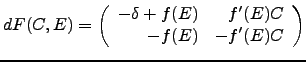 |
(2.7) |
| (2.8) |
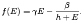
Thus, since ![]() , the cell production rate is diminished by the need to produce
the ECM component.
In the expression for
, the cell production rate is diminished by the need to produce
the ECM component.
In the expression for ![]() ,
parameters
,
parameters ![]() and
and ![]() describe the cell-matrix interaction
that affects proliferation of both
describe the cell-matrix interaction
that affects proliferation of both ![]() and
and ![]() ,
and parameter
,
and parameter ![]() is the ``treshhold'' parameter describing where the
negative feedback control in the production of ECM is ``switched on''.
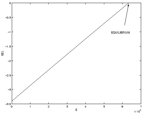
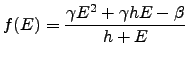
More precisely, the expression
is the ``treshhold'' parameter describing where the
negative feedback control in the production of ECM is ``switched on''.
More precisely, the expression
![]() , which determines,
among other things, the generation rate of ECM, will be influenced to
the ``leading order'' only after
, which determines,
among other things, the generation rate of ECM, will be influenced to
the ``leading order'' only after ![]() reaches the treshold value of
reaches the treshold value of ![]() .
A typical graph of
.
A typical graph of ![]() is given in Figure 2.1.
is given in Figure 2.1.
The non-dimensional form of the above system is obtained by the following scalings of the variables
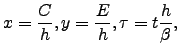 |
(2.9) |
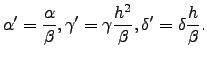 |
(2.10) |
This model is similar to that proposed in [5] to study the dynamics of cell and extracellular matrix. The model in [5], however, gives rise to the equilibrium that is a spiral sink for the data of our interest. This would mean, in particular, that the concentrations of chondrocytes and ECM approached the equilibrium in an oscillatory fashion, which was not observed in our experiments. In particular, the model proposed in [5] showed a region of decrease in the concentration of ECM in the intermediate stage of the ECM development, indicating degradation of ECM, not experimentally observed or justified. Never the less, the model in [5] provided a guidance for the development of the model in the present manuscript.
In the next section we show
how experimental results compare with
the numerical simulations of the model (2.1)-(2.3),
showing excellent agreement.
Additionally, we shall see that the parameters that determine
the cell proliferation rate on a particular artificial surface
are ![]() and
and ![]() . In fact, it is the ratio
. In fact, it is the ratio
![]() that determines the artificial surface-dependent cell proliferation rate.
High ratio
that determines the artificial surface-dependent cell proliferation rate.
High ratio
![]() means highly condusive artificial surface.
means highly condusive artificial surface.