M.A.Olshanskii

Free surfice flows of visco-plastic fluids

Visco-plastic fluids combine solid-like behavior in the absence of intervention and fluid-like response at stress. The shift between this two conditions is formalized by yield stress parameter.

Collaborators:

Kirill Nikitin (INM RAS)

Kirill Terekhov (INM RAS)

Yuri Vassilevski (INM RAS)

Ruslan Yanbarisov (INM RAS)

Wanli Cheng (former University of Houston)

A model for free-surface viscoplastic fluid flow

Fluid domain: $\Omega(t)\in\mathbb{R}^3$ with boundary $\overline{\partial \Omega(t)}=\overline{\Gamma_D}\cup\overline{\Gamma(t)}$
$\Gamma_D$: solid part, $\; \Gamma(t)$: free surface

Fluid equations:
$$ \left\{ \begin{split} \rho\left(\frac{\partial {\mathbf{u}}}{\partial t}+ ({\mathbf{u}} \cdot \nabla) {\mathbf{u}}\right) -\bf{div}\,\tau + \nabla p = {\bf f}\\ \nabla \cdot {\mathbf{u}} = 0 \end{split}\right. \quad\text{in}~ \Omega(t), $$

The Herschel-Bulkley constitutive law:
\begin{equation*} \begin{split} \mathbf{\tau} = \left(K\,|\mathbf{Du}|^{n-1} + \tau_s |\mathbf{Du}|^{-1}\right)\mathbf{Du}&~ \Leftrightarrow~ |\tau| > \tau_s,\\ \mathbf{Du} = \mathbf{0}&~ \Leftrightarrow~ |\tau|\le \tau_s. \end{split} \end{equation*}

$K>0$: consistency parameter,
$\rho$: density of fluid,
$\bf{Du}=\frac{1}{2}[\nabla\mathbf{u} + (\nabla\mathbf{u})^T]$: rate of strain tensor,
$\tau$: deviatoric part of the stress tensor,

$\tau_s\ge0$: yield stress parameter,
$\bf{u}$: velocity vector,
$n>0$: flow index,
p: kinematic pressure.

For a passively advected free surface $\Gamma(t)$, it holds $ v_{\Gamma} = \mathbf{u}|_{\Gamma} \cdot \mathbf{n}_{\Gamma}, $ where $\mathbf{n}_{\Gamma}$ is the normal vector for $\Gamma(t)$ and $v_{\Gamma}$ is the normal velocity of $\Gamma(t)$. The balance the surface tension and stress forces gives the second condition on $\Gamma(t)$ : \begin{equation*}\label{eq:tension} \boldsymbol{\sigma} \mathbf{n}_{\Gamma} = \varsigma \kappa \mathbf{n}_{\Gamma} %- p_{\rm ext} \mathbf{n}_{\Gamma} \quad\text{on}~ \Gamma(t), \end{equation*} $\kappa$ is the sum of the principal curvatures, $\varsigma$ is the surface tension coefficient.

Do not forget initial and boundary conditions. :-)

Examples and illustrations

Computational Herschel-Bulkley fluid flows

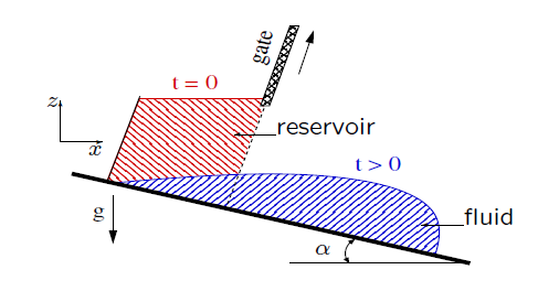
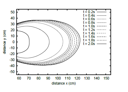
The sketch of the flow set-up: viscoplastic fluid flows over incline planes; see [7].

Flow animation: viscoplastic fluid flows over incline planes.
Plots: evolution of the contact line of the free-surface.
Parameters: $\alpha=12^o$, $K\,=47.68 Pa s^{-n}$, $n=0.415$, $\tau_s=89 Pa$.

Compare the numerics with the report of Cochard and Ancey on experimental studies with Carbopol Ultrez 10 gel (flow over an inclined plane, same set-up): "... we observed two regimes: at the very beginning ($t<1s$), the flow was in an inertial regime; the front velocity was nearly constant. Then, quite abruptly, a pseudo-equilibrium regime occurred, for which the front velocity decayed as a power-law function of time."

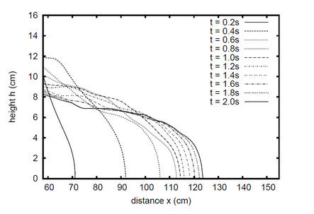
Flow animation: viscoplastic fluid flows over incline planes. The opening gate is now simulated numerically.
Plots: evolution of the midplane flow-depth profile.
Parameters: $\alpha=12^o$, $K\,=47.68 Pa s^{-n}$, $n=0.415$, $\tau_s=89 Pa$.

Computations for Herschel-Bulkley fluid, $n=1\Rightarrow$ Bingham

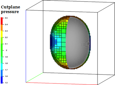
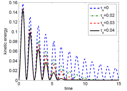
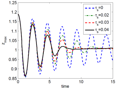
Freely oscillating droplet problem; see [2] and [7].

Viscoplastic case, $\tau_s>0 \qquad \Longrightarrow \qquad $ Finite cessation times?

The kinetic energy decay (left) and top tip trajectories (right) for different stress yield parameter values, $$\tau_s\in\{0,\, 0.02,\, 0.03,\, 0.04\}:$$

Few more animations of complex and/or entertaining
fluid flows (computed and rendered by Kirill Nikitin)

For algorithms description see [3-6].

Newtonian fluids:

Sayana-Shushenskaya Dam Break (Newtonian fluid):

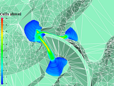
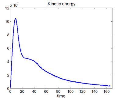
Sayana-Shushenskaya Landslide (Herschel-Bulkley fluid). Landslide run-out and kinetic energy evolution:
(real-life topography thanks to Shuttle Radar Topography Mission (NASA))

(H.-B. model coefficients correspond to rheology of Puglia mountains landslides.)

Metro station from "Moscow 2033" novel:

The bibliography

K.D. Nikitin, M.A. Olshanskii, K.M. Terekhov, Yu.V. Vassilevski, R. Yanbarisov, An adaptive numerical method for free surface flows passing rigidly mounted obstacles, Computers & Fluids, V. 148 (2017), 56-68, pdf-file;

W. Cheng, M.A. Olshanskii, Finite stopping times for freely oscillating drop of a yield stress fluid, Journal of Non-Newtonian Fluid Mechanics 239 (2017), 73-84, pdf-file;

K.M. Terekhov, K.D. Nikitin, M.A. Olshanskii, Y.V.. Vassilevski, A semi-Largangian method on dynamically adapted octree meshes, Rus.J.Num.Anal.Math.Model. 30 (2015), 363-380, pdf-file;

K.D. Nikitin, M.A. Olshanskii, K.M. Terekhov, Yu.V. Vassilevski, A splitting method for numerical simulation of free surface flows of incompressible fluids with surface tension, Computational Methods in Applied Mathematics , 15 (2015), 59-77, pdf-file

M.A. Olshanskii, K.M. Terekhov, Y.V. Vassilevski, An octree-based solver for the incompressible Navier-Stokes equations with enhanced stability and low dissipation, Computers & Fluids, 84 (2013), 231-246, pdf-file

K.D. Nikitin, M.A. Olshanskii, K.M. Terekhov, Yu.V. Vassilevski, A CFD approach to the 3D modelling of large-scale hydrodynamic events and disasters, Rus.J.Num.Anal.Math.Model., 27 (2012), 399-412, pdf-file;

K.D. Nikitin, M.A. Olshanskii, K.M. Terekhov, Yu.V. Vassilevski,
A numerical method for the simulation of free surface flows of viscoplastic fluid in 3D, J.Comp.Math., 29 (2011), 605-622, pdf-file;