Trace finite element method
Trace finite element method is a technique for solving PDEs on curvilinear (evolving) geometries without mesh fitting and geometry parametrization.
Collaborators:
Alexey Chernyshenko (INM RAS, Moscow)
review paper: M.A. Olshanskii, A. Reusken, Trace Finite Element Methods for PDEs on Surfaces, pdf-file;
Example of a problem setup: For a given vector field $\mathbf{w}$ in $\Omega\subset\mathbb{R}^3$, a surface $\Gamma(t)\subset\Omega$ evolves with the normal velocity $\mathbf{w}\cdot\mathbf{n}_\Gamma$. The conservation of a scalar quantity $u$ with a diffusive flux on $\Gamma(t)$ leads to the surface PDE: \[ \dot{u} + ({\bf div}_{\Gamma}\mathbf{w})u -\varepsilon\Delta_{\Gamma} u=0\qquad\text{on}~~\Gamma(t),~~~~~~~~~~~(1) \] $\varepsilon$ is the diffusion parameter, $\dot{u}$ is material derivative.
Numerical simulation of transport and diffusion along two colliding droplets:
Color shows the concentration (of a surfactant) on the droplets surface. The numerical example is taken from [8]. Equations (1) are solved by the space-time trace FEM from [6,7].
PDEs on surfaces arise in several application:
- Transport and diffusion of surfactants on multiphase flow interfaces (e.g. pulmonary surfactants are critical for reduction of fluid in lungs surface tension and increase pulmonary compliance);
- Diffusion of transmembrane receptors and signalling molecules along cell membranes;
- Biological pattern formation (e.g. Turing patterns on surfaces);
- etc.
|
The idea behind the method: Take all finite element functions for a bulk geometry-independent triangulation and consider their traces on a reconstructed domain of interest (surface or embedded volumetric domain). |
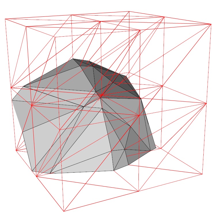
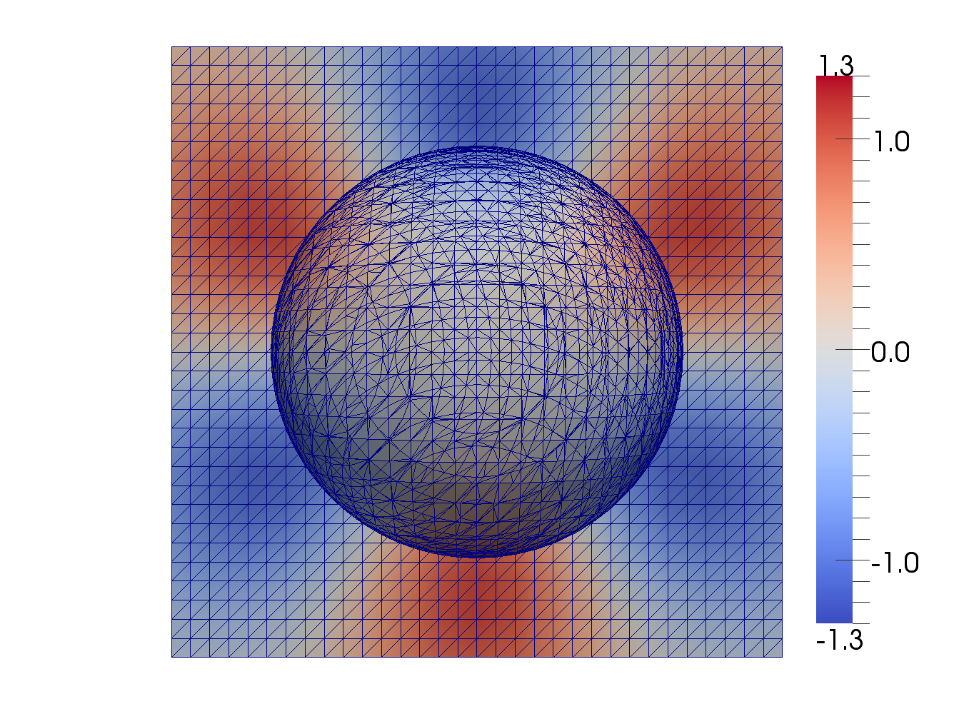
For the illustration, consider the Laplace-Beltrami equation on the unit sphere \[ -\Delta_\Gamma u + u =f\quad\mbox{on}~\Gamma=\{ \mathbf{x}\in\mathbb{R}^3\mid \|\mathbf{x}\|_2 = 1\}, \] and a regular tetrahedral triangulation of $\Omega= (-2,\,2)^3$.
Let $~\phi_h:=I(\phi)$ be a piecewise linear continuous interpolant of $\phi(\mathbf{x})=\|\mathbf{x}\|^2-1$.
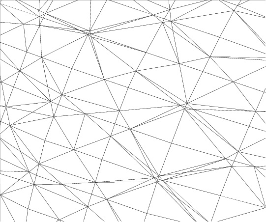
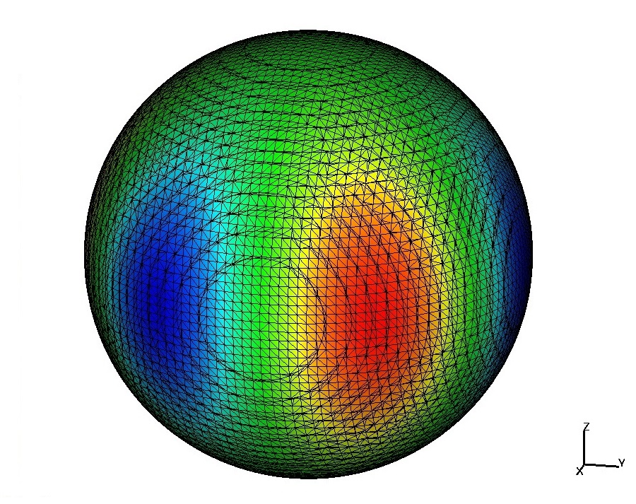
The pictures below illustrate a part of the reconstructed surface \[ \Gamma_{h}:= \{ \, \mathbf{x} \in \Omega ~|~ \phi_h(\mathbf{x})=0 \, \}. \] and a piece of the induced trace triangulation, and a computed solution colored over $\Gamma_{h}$.
|
|
|
| Reconstructed surface | Irregular trace triangulation | Computed solution |
The interface triangulation $\Gamma_h$ is not shape-regular (interesting properties of trace triangulations are studied in [4]), however the method is numerically stable and convergence rates are optimal.
More examples
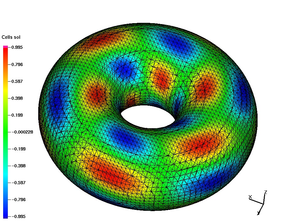
Smooth solution on a torus
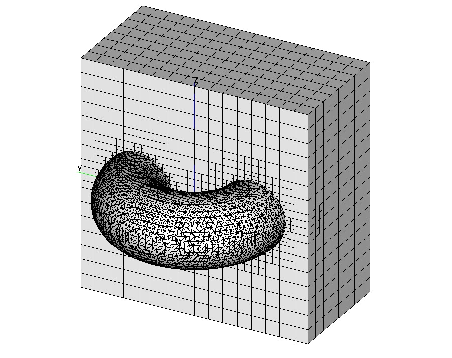
The Laplace-Beltrami type equation on the torus: \[ -\Delta_\Gamma u +u =f\quad\mbox{on}~\Gamma,~~\Gamma\subset\Omega=(-2,2)^3, \] with $\Gamma = \{ {\bf x}\in\Omega \mid r^2 = x_3^2 + (\sqrt{x_1^2 + x_2^2} - R)^2\}$, $R= 1$ and $r=0.6$. In the coordinate system $(\rho, \phi,\theta)$, with \[ {\bf x} = R\begin{pmatrix}\cos\phi \\ \sin\phi \\ 0 \end{pmatrix} + \rho\begin{pmatrix}\cos\phi\cos\theta \\ \sin\phi\cos\theta \\ \sin\theta \end{pmatrix}, \] the solution $u$ and the right-hand side are taken as: \begin{equation}\label{polar2} \begin{split} u({\bf x})&= \sin(3\phi)\cos( 3\theta + \phi),\\ f({\bf x})&= r^{-2} (9\sin( 3\phi)\cos( 3\theta + \phi)) - (R + r\cos( \theta))^{-2}(-10\sin( 3\phi)\cos(3\theta + \phi) - 6\cos( 3\phi)\sin( 3\theta + \phi)) \\ & \quad -(r(R + r\cos( \theta))^{-1}(3\sin( \theta)\sin( 3\phi)\sin( 3\theta + \phi))+u({\bf x}). \end{split} \end{equation} The trace FEM works with various bulk (unfitted) meshes. The above example used a tetrahedra subdivision. Below we use octree grids and P1 continuous bulk finite elements. Discontinuous Galerkin trace method is another option here.
|
|
| Bulk octree grid and induced surface meshes | Computed solution |
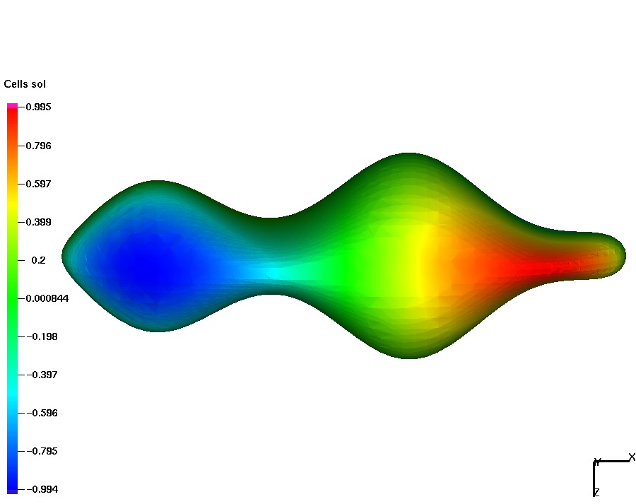
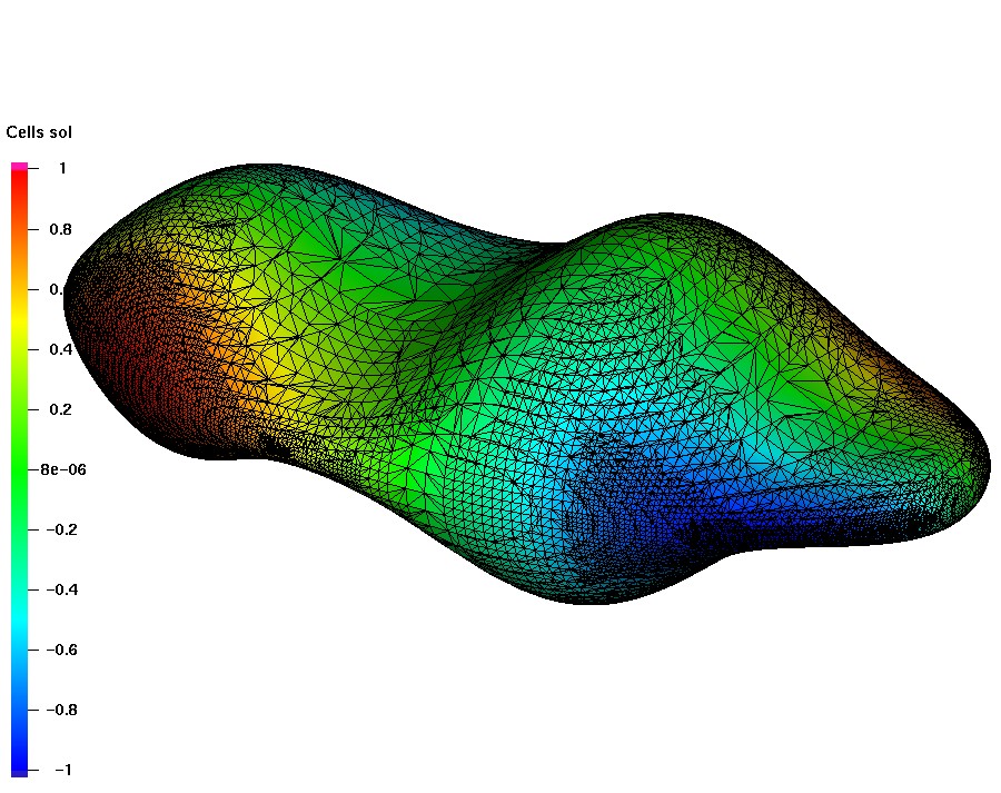
Laplace-Beltrami eq. on a different shape I
The surface is given by the zero of the level set function \[ \phi({\bf x})=\frac14 x_1^2+x_2^2+\frac{4x_3^2}{(1+\frac12\sin(\pi x_1))^2}-1. \] The Laplace-Beltrami equation is solved for the exact solution $u=x_1x_2$ on $\Gamma$. To compute the corresponding right-hand side, consider the normal vector ${\bf n}=\nabla\phi/|\nabla\phi|=:(n_1,n_2,n_3)^T$ on $\Gamma$ and the Weingarten map ${\bf H}=\nabla_\Gamma{\bf n}$ with its entries given by \[ {\bf H}_{im}=\frac1{|\nabla\phi|}\left(\phi_{x_ix_m} -\frac{\phi_{x_i}(\sum_{k=1}^3\phi_{x_k}\phi_{x_kx_m})+\phi_{x_m}(\sum_{j=1}^3\phi_{x_j}\phi_{x_ix_j})}{|\nabla\phi|^2} +\frac{\phi_{x_i}\phi_{x_m}(\sum_{j=1}^3\sum_{k=1}^3\phi_{x_k}\phi_{x_kx_j})}{|\nabla\phi|^4}\right) \] for $i,m=1,2,3$. The right-hand side is \[ f({\bf x})=x_1x_2+2n_1({\bf x})n_2({\bf x})+\mbox{tr}({\bf H}({\bf x}))(x_1n_2({\bf x})+x_2n_1({\bf x})),\quad{\bf x}\in\Gamma. \]
|
|
| Smooth solution | Numerical solution |
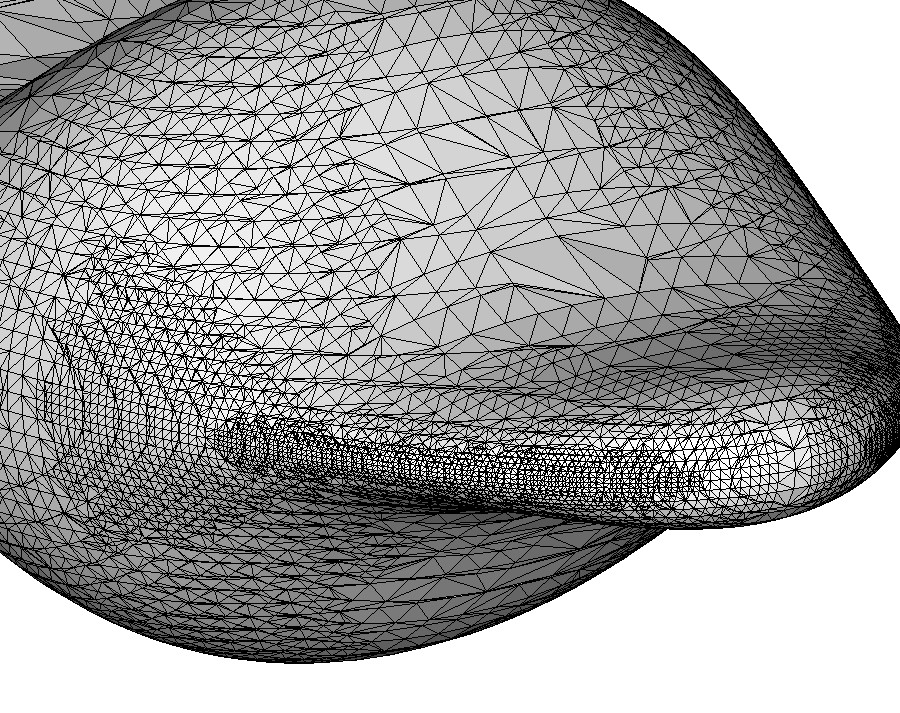
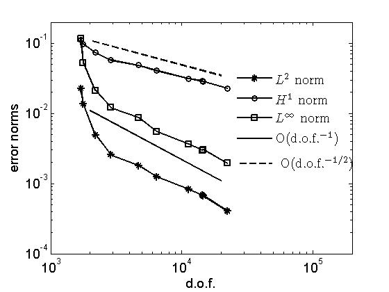
The figure above shows the numerical solution and plots it over the trace mesh, which results after 9 steps of adaptation, starting with the uniform cubic mesh with $h=1/4$. The mesh adaptation is based on a residual error indicator, which also accounts for geometric errors, see [3,11]. The optimal convergence order with respect to the total number of degrees of freedom in $L^2$, $H^1$ and $L^\infty$ surface norms is shown below (see the references for examples with singular solutions).
|
|
| The plot zooms the trace surface mesh | Error reduction for adaptive grid refinement |
Laplace-Beltrami eq. on a different shape II
The surface is given implicitly as the zero level set of \[ \phi=(x_1^2+x_2^2-4)^2+(x_2^2-1)^2+(x_2^2+x_3^2-4)^2+(x_1^2-1)^2+(x_1^2+x_3^2-4)^2+(x_3^2-1)^2-13. \] and it is homeomorphic to the sphere with 6 handles.
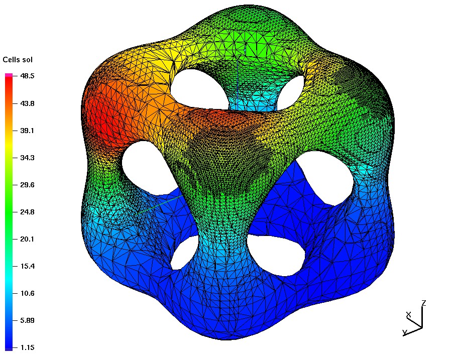
The figure shows a computed solution to the Laplace-Beltrami equation for $f=100\sum_{j=1}^4\exp{(-|{\bf x}-{\bf x}^j|^2)}$, with \[ {\bf x}^1=(-1,1,2.04),~~ {\bf x}^2=(1,2.04,1),~~ %\\[1ex] {\bf x}^3=(2.04,0,1),~~ {\bf x}^4=(-0.-1,-2.04). \] The points are close to the surface and the right-hand side is varying rapidly in vicinities of these 4 points, and hence the same is expected from the solution. The visualized grid results after 12 steps of adaptive refinement.
Transport and diffusion with a layer fitted mesh
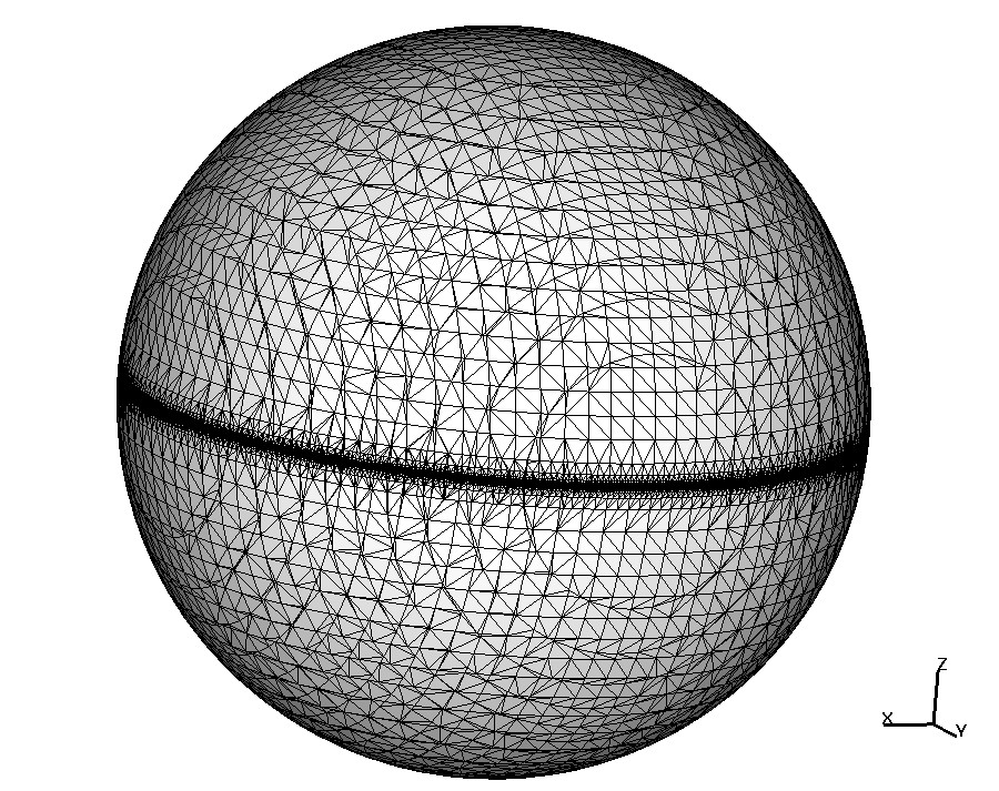
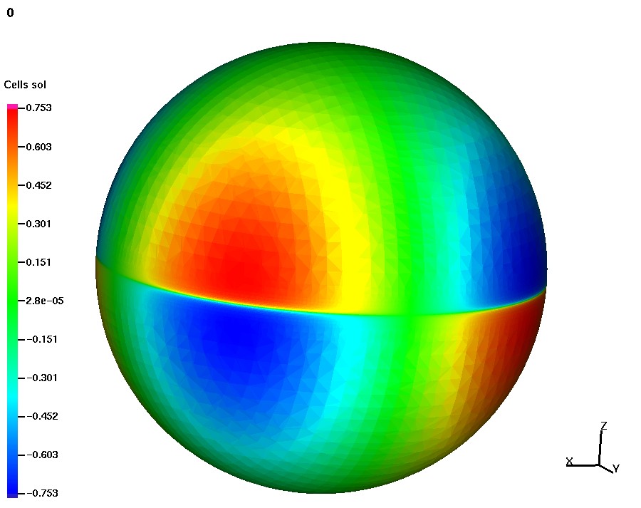
The steady advection-diffusion equation \[ -\varepsilon\Delta_{\Gamma} u+\mathbf{w}\cdot\nabla_{\Gamma} u + (c+{\bf div}_\Gamma{\bf w})\, u =f\quad\text{on the unit sphere} \] is solved for the solution \[ u(\bf x)= {x_1 x_2}\mathrm{arctan}\left(\frac{2x_3}{\sqrt{\varepsilon}}\right). \] For $\varepsilon=1e-4$ the problem is transport dominated and the solution has a $O(\sqrt{\varepsilon})$ internal layer along the equator. The trace FEM is convenient for using layer adapted meshes.
|
|
| Shishkin trace mesh | Computed solution |
The figure shows the trace of octree Shishkin mesh adapted towards the layer and the computed solution with internal layer resolved. Error reduction on a sequence of layer adapted mesh is optimal w.r.t. the number of active d.o.f., see [11]. Another option for transport dominated problems is to use upwind/ Petrov-Galerkin methods. This is also easily done in the framework of trace FEN, see [5].
Bulk-surface coupled problems
Transport and diffusion in a volume and on interface in an equilibrium: \[ \begin{aligned} - \nu_i\Delta u_i + \mathbf{w} \cdot \nabla u_i & = f_i \quad \text{in}~ \Omega_i, ~i=1,2, \\ - \nu_\Gamma \Delta_\Gamma v + \mathbf{w} \cdot \nabla_\Gamma v + K[ \nu \mathbf{n} \cdot \nabla u]_\Gamma& = g \quad \text{on}~~\Gamma, \\ (-1)^{i} \nu_i \mathbf{n} \cdot \nabla u_i & = u_i- q_i v \quad \text{on}~~\Gamma, \quad i=1,2, \\ \mathbf{n}_{\Omega} \cdot \nabla u_2 & =0 \quad \text{on}~~\partial \Omega, \\ \text{with} ~~q_i & := \frac{ k_{i,d}}{ k_{1,a}+ k_{2,a}} \in [0,1]. \end{aligned} \] The Henry law is assumed for absorbtion and desorption on an interface.
The figure illustrates the mesh in a volume on an interface and computed solution, see [10] for the analysis and experiments with the coupled surface-bulk trace FEM.
Transport-diffusion in fractured porous media
The scope of this research is to simulate transport and diffusion in fractured porous media, using monotone FV schemes with multipoint flux approximation for the transport and diffusion in the bulk and trace FEM for the transport and diffusion in the fractures. The system of equations is given by \[ \left\{ \begin{aligned} \phi_i\frac{\partial u_i}{\partial t} + {\bf div}(\mathbf{w}_i u_i)- D_i \Delta u_i &= f_i \quad \text{in}~ \Omega_i,\\ u_i&=v \quad \text{on}~ \partial\Omega_i\cap\Gamma, \end{aligned} \right. \] and on the surface, \[ \label{diffeq2} \phi_\Gamma\frac{\partial v}{\partial t} + {\bf div}_\Gamma (\mathbf{w}_\Gamma v) - d D_\Gamma \Delta_\Gamma v = F_\Gamma(u)+ f_\Gamma \quad \text{on}~~\Gamma, \] where $F_\Gamma(u)$ stands for the net flux of the solute per surface area due to fluid leakage and hydrodynamic dispersion; $f_i$ and $f_\Gamma$ are given source terms in the subdomains and in the fracture; $D_i >0$ denotes the diffusion coefficient for the porous matrix, which is assumed to be constant in $\Omega_i$; the surface diffusion coefficient $D_\Gamma >0$ and the fracture width coefficient $d>0$ may vary along $\Gamma$; $\phi_i>0$ and $\phi_\Gamma>0$ are the constant porosity coefficients for the bulk and the fracture. The total surface flux $F_\Gamma(u)$ represents the contribution of the bulk to the solute transport in the fracture. The mass balance at $\Gamma$ leads to the equation \[ F_\Gamma(u)= [-D {\mathbf n} \cdot \nabla u + ({\mathbf n} \cdot{\mathbf w})u]_\Gamma, \] where ${\mathbf n}$ is a unit normal vector at $\Gamma$, $[w({\mathbf x})]_\Gamma$, ${\mathbf x}\in\Gamma$, denotes the jump of $w$ across $\Gamma$ in the direction of ${\mathbf n}$.
Cutaway of a bulk domain with an embedded branching fracture. The color shows the transport and diffusion of a solute concentration in the bulk and along the fracture. Computed with the hybrid Finite Volume -- TraceFEM method from [13].
Summary of the Trace FEM:
The method is based on traces of outer finite element spaces.
- It is essentially Eulerian: $\Gamma$ is not tracked by a mesh;
- If $\Gamma$ evolves, one recomputes matrices, using the same data structures;
- No extension of equation from the surface is needed;
- Number of active degrees of freedom is optimal, it is comparable to methods in which $\Gamma$ is meshed directly;
- Optimal order of convergence in $H^1$ and $L^2$ norms;
- Reliable error indicators are available;
- Amenable for both space and time adaptivity;
- After suitable stabilization, effective condition numbers of matrices are comparable to common FE;
- Numerical analysis is rather challenging, but now well developed.
Learn about some applications of Trace FEM:
The bibliography
(this is by no means complete list of papers on TraceFEM; it collects only papers I am co-authoring)- M.A. Olshanskii, A. Reusken, J. Grande,
A Finite Element method for elliptic equations on surfaces, SIAM J. Numer. Anal. V.47 (2009), 3339-3358; pdf-file - M.A. Olshanskii, A. Reusken,
A finite element method for surface PDEs: Matrix properties, Numerische Mathematik V. 114 (2010), 491-520; pdf-file - A. Demlow, M.A. Olshanskii,
An adaptive surface finite element method based on volume meshes, SIAM J. Numer. Anal. V. 50 (2012), 1624-1647; pdf-file - M.A. Olshanskii, A. Reusken, X. Xu,
On surface meshes induced by level set functions, Computing and Visualization in Science V. 15 (2013), 53-60; pdf-file - M.A. Olshanskii, A. Reusken, X. Xu,
A stabilized finite element method for advection-diffusion equations on surfaces, IMA J Numer. Anal. V. 28 (2014), 732-758; pdf-file - M.A. Olshanskii, A. Reusken, X. Xu,
An Eulerian space-time finite element method for diffusion problems on evolving surfaces, SIAM J. Numer. Anal. V. 52 (2014), 1354-1377; pdf-file - M.A. Olshanskii, A. Reusken,
Error analysis of a space-time finite element method for solving PDEs on evolving surfaces, SIAM J. Numer. Anal. V. 52 (2014), 2092-2120; pdf-file - J. Grande, M.A. Olshanskii, A. Reusken,
A space-time FEM for PDEs on evolving surfaces, in proceedings of 11th World Congress on Computational Mechanics (2014), E. Onate, J. Oliver and A. Huerta (Eds), pdf-file - M.A. Olshanskii, D. Safin,
A narrow-band unfitted finite element method for elliptic PDEs posed on surfaces, Mathematics of Computation, V. 85 (2016), 1549-1570, DOI: 10.1090/mcom/3030, pdf-file - S. Gross, M.A. Olshanskii, A. Reusken,
A trace finite element method for a class of coupled bulk-interface transport problems, ESAIM: Mathematical Modelling and Numerical Analysis, V. 49 (2015), 1303-1330, pdf-file - A. Chernyshenko, M.A. Olshanskii,
An adaptive octree finite element method for PDEs posed on surfaces, Comp.Meth.Appl.Mech.Eng., V. 291 (2015), 146-172, pdf-file - M.A. Olshanskii, D. Safin, Numerical integration over implicitly defined domains for higher order unfitted finite element methods, Lobachevskii Journal of Mathematics, V. 37 (2016), 582-596, pdf-file
- A.Y. Chernyshenko, M.A. Olshanskii, Yu.V. Vassilevski, A hybrid finite volume-finite element method for bulk-surface coupled problems, Journal of Computational Physics, V. 352 (2018), 516-533, pdf-file;
- M.A. Olshanskii, X. Xu, A trace finite element method for PDEs on evolving surfaces, SIAM J.Sci.Comp. V. 39 (2017), A1301-A1319 pdf-file;
- review paper: M.A. Olshanskii, A. Reusken, Trace Finite Element Methods for PDEs on Surfaces, in Lecture Notes in Computational Science and Engineering series, V. 121 (2018), 211--258, pdf-file;
- S. Groß, T. Jankuhn, M. Olshanskii, A. Reusken, A Trace Finite Element Method for Vector-Laplacians on Surfaces, SIAM J.Numer.Anal. V. 56 (2018), 2406-2429, pdf-file;
- C. Lehrenfeld, M. Olshanskii, X. Xu, A stabilized trace finite element method for partial differential equations on evolving surfaces, SIAM J.Numer.Anal. V. 56 (2018), 1643-1672, pdf-file;
- A. Chernyshenko, M. Olshanskii, An unfitted finite element method for the Darcy problem in a fracture network, Journal of Computational and Applied Mathematics; V. 336 (2020), Article 112424; doi:10.1016/j.cam.2019.112424; pdf-file
**Past and current support acknowledgment: NSF through the Division of Mathematical Sciences grant 1315993 and 1717516.